In the previous post, I explained the idea behind cascade classifiers. In this post, I will give you some clear instructions to easily train an accurate custom object detector using my C++ toolbox. We will see how easily we can accelerate this accurate detector by 20%. Stay tuned :)

­

LBP Cascade running on Odroid XU4 

­

1. How to train your custom model with my toolbox?

OpenCV 2 and 3 provide some executables to train a cascade classifier. These executables are well documented but I found them hard-to-use in real-world applications in which training starts with an initial data and must be repeated over and over again when new data is added for the sake of accuracy. So, I made a toolbox to make the process easier. There are separate apps for collecting train/test data, training the model, testing it, and do hard negative mining (I will explain this a few minutes later).

To build an accurate detector:

git clone https://github.com/zanazakaryaie/Detection_Toolbox.git
cd Detection_Toolbox
mkdir build && cd build
cmake ..
make

Then use the generated executables in the following order:

1.1– collect_train_data

Training a cascade classifier requires positive and negative images. Positive images are the ones that contain your desired object with some background (max. 10%). Negative images are the ones that contain anything except your desired object. It’s very important to collect negative images from the scenes where you want to later run your detector, instead of collecting random images from Google!

If you have previously collected positive and negative images in separate directories, then skip this step. If not, run collect_train_data. It creates two folders. One for positive images and the other for negatives. It then asks you to select a video file that contains your object. A window pops-up showing the first frame of the video. Draw a rectangle over your object by pressing left-click on its top-left corner dragging to the bottom-right corner. Release the left-click to finish the drawing. You can edit the rectangle by left-clicking on the anchors to move them. Add other existing objects in the frame. Notice that the objects must have similar aspect ratios. This is the limitation of the cascade classifier. If you want to delete an object, right-click inside it. Once finished annotating all the objects in the first frame, press space to move 10 frames forward. You can increase or decrease the step by pressing “+” or “-” on your keyboard. The annotation continues until reaching the end of the video or whenever you press the “q” button. The average aspect ratio is reported at the end. We need this number in step 1.3. The objects you annotated are put in the positive folder. Negative images are automatically generated by cropping random regions of the annotated frames (positives excluded). To make sure that the generated negative images do not contain any positive samples, go to the negative folder and remove all images that contain positive samples. This is very very important.

1.2- collect_test_data

To later assess our trained model, we need to collect some test data. Run ./collect_test_data and select a video file. A window pops-up showing the first frame of the video. Do exactly the same works in step 1.1. A folder is created that saves the annotations of each frame in separate .txt files. We will use these files in step 1.4.

1.3– train

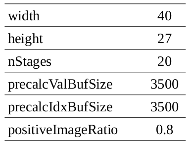
Once the positive and negative images are prepared in their directories (from step 1.1), open params/configs.yaml, and edit the parameters:

• width–height: width and height of the sliding window.

  You can’t detect an object that is smaller than width*height. Higher values allow more features to be extracted. This can increase the accuracy but also increases the training and inference times exponentially. The width/height ratio must be the same as the ratio reported in step 1.1, otherwise, the positive images are stretched and the accuracy is reduced.

• featureType: LBP or HAAR.

  LBP is much faster to train and execute but has a lower accuracy than HAAR. We will see the comparison in a few minutes.

• nStages: the number of weak classifier stages.

  The more stages, the longer the training process takes (exponentially). Set this to a number between 15-20. Whenever the acceptance ratio reaches 10^(-5), press ctrl+c to stop the training, otherwise your classifier becomes over-fitted.

• precalcValBufSize: RAM size in MB dedicated for calculating the feature values. Increase it to lower the training time.

• precalcIdxBufSize: RAM size in MB dedicated for calculating the feature indices. Increase it to lower the training time.

• positiveImageRatio: Set this to a number between 0.7-0.8.

  The classifier starts with this ratio of the positive images. The remaining positives are only used if the classifier requires them in the later stages. Higher values (e.g. 0.9) might raise an error during training (explained in a few seconds).

close the configs.yaml and run ./train. It asks you to select the configs file, and positive and negative directories respectively. Wait for the training to finish. It takes time depending on the featureType, nStages, and the number of images you feed for training. If either you stop the training (by pressing ctrl+c) or the training itself stops before reaching nStages, then the program generates the model up to the last available stage. The following list explains the possible reasons that the training stops before reaching the number of the determined stages:

1. Required leaf false alarm rate achieved. Branch training terminated.

        You must feed more negatives (if the acceptance ratio has not achieved 10^(-5)).

2. Can not get new positive sample. The most possible reason is insufficient count of samples in given vec-file.

        You must reduce the “positiveImageRatio” to allow the algorithm to get new positive samples.

1.4– test

After training has finished, run ./test to see the accuracy of the trained model. Select the test video file, the trained cascade model, and the TestData directory (generated from step 1.2) respectively. A window pops-up showing the detected objects (in blue) and the ground truth objects (in green). The precision and recall are then calculated according to the following equations:

Precision = TP/(TP+FP)

Recall = TP(TP+FN)

where TP stands for the true positives, FP for the false positives, and FN for the false negatives.

1.5– hard_negative_mine

When testing a model, it’s quite expected that you see lots of false positives. This goes back to the idea behind a cascaded classifier. Each stage must have a very low false negative rate but can have false positive rates because later stages can correct it.

To make your model more accurate, you must add those false positives to the list of negative images and retrain your model. This is called hard negative mining. To do this, run ./hard_negative_mine and select your train video. A window pops-up showing the first frame. Right-click inside each false positive to add it to the folder of negatives. Leave the true positives and draw false negatives if required (they will be added to the positive folder). When finished, press space to move to the next 10th frame. This continues until reaching the end of the test video or whenever you press the “q” button.

1.6– Go to 1.3 and repeat

Now that the new negatives and positives have been added to their folders, train a new cascade, and again check its accuracy on your test data. You may need to do hard negative mining for two or three times to achieve satisfactory results.

­

2. Example: racecar detection in Gran Turismo game!

I downloaded a Gran Turismo video from Youtube and split it into 2 videos. One before pit-stop (18:04) for training, and the other after pit-stop (18:18) for testing. I used collect_train_data to collect 424 positive and 848 negative images. Then I used collect_test_data to annotate 100 frames. It took 12 minutes to train a HAAR model, and 5 minutes to train an LBP model on an Intel(R) Core(TM) i7-5600U CPU @ 2.60GHz with 8GB of DDR3 RAM.

­

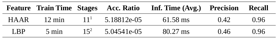
1. Training finished with this message: “Required leaf false alarm rate achieved. Branch training terminated.”

2. I stopped training at this stage because the acceptance ratio reached near the HAAR’s ratio. This allows for fair accuracy comparison.

­

To increase accuracy, I used the LBP model in hard_negative_mine and collected 900 more negatives. See the results of the re-trained models.

­

­

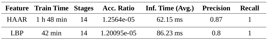
The HAAR model is more accurate. It doesn’t miss any car in the test data (Recall: 1) but has few false positives. Also, the inference time is almost half of the LBP model (I didn’t expect this myself). The only drawback is it’s longer training time. However, it can be significantly reduced if you have more RAM. I had 8GB of RAM but allocated 4GB of swap memory to avoid crash when training. This was the main reason for such slow training.

The reason behind the higher accuracy of the HAAR model is that it can extract much more unique features from a 40×27 window. HAAR extracts 567460 features while LBP extracts 30420 ones.

­

3. Accelerate it!

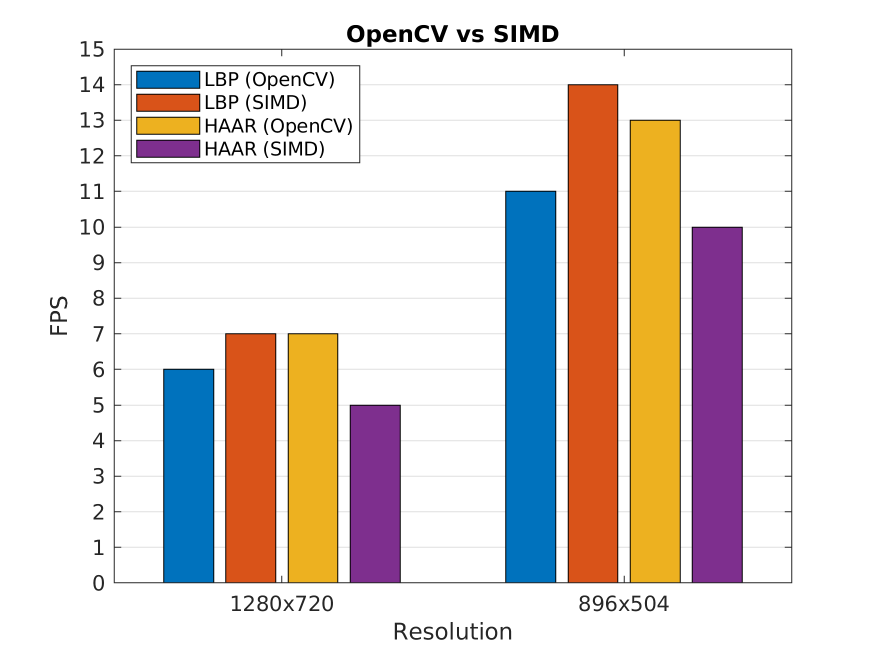
Simd is a good library developed for accelerating image processing algorithms using vectorization. It supports both X86 and ARM intrinsics. You can easily accelerate the inference time of your cascade model using this library and a few lines of code:

#include <opencv2/opencv.hpp>
#include <chrono>
#define SIMD_OPENCV_ENABLE
#include <Simd/SimdDetection.hpp>
#include "utils.hpp"

using namespace cv;
using namespace std;

int main()
{
    string videoName = selectFile("Select Video File", {"*.mp4", "*.avi"});
    VideoCapture cap(videoName);

    string modelName = selectFile("Select Cascade Model", {"*.xml"});

    typedef Simd::Detection<Simd::Allocator> Detection;

    Detection detection;
    detection.Load(modelName);

    bool inited = false;

    while (cap.isOpened())
    {
        Mat frame;
        cap.read(frame);

        if (frame.empty())
            break;

        Detection::View image = frame;

        auto t1 = std::chrono::high_resolution_clock::now();

        if (!inited)
        {
            detection.Init(image.Size(), 1.1);
            inited = true;
        }

        Detection::Objects objects;
        detection.Detect(image, objects);

        auto t2 = std::chrono::high_resolution_clock::now();
        int duration = std::chrono::duration_cast<std::chrono::milliseconds>( t2 - t1 ).count();

        for (const auto& object:objects)
            rectangle(frame, object.rect, Scalar(0,255,0), 3);

        ostringstream FPS;
        FPS << "FPS: " << 1000/duration;
        putText(frame, FPS.str(), Point(10,30), 0, 1, Scalar(0,0,255), 2);

        imshow("Detections", frame);

        if (waitKey(1)=='q')
            break;
    }

    cap.release();

    return 0;
}

See the gain with different image resolutions on Odroid XU4.

4. Limitations

As mentioned in the previous post, the cascade classifier works on rigid objects. If you want to detect multiple classes of objects with different aspect ratios (e.g. cars and pedestrians), then you have to train a separate model for each class. This makes it unsuitable because the runtime increases significantly. However, if you want to detect multiple classes of similar objects with the same aspect ratios (e.g. cars, vans, and pickups in rear-view), then cascade can do the job. You would better think of this algorithm as an object categorizer rather than an object detector.

Another limitation is that the algorithm is not rotation invariant. Research has proven that a single model can handle -10 to +10 degrees. If you want more invariance, you have to either train separate models for different rotation bins or alternatively rotate the input image with different angles and aggregate the outputs of running the model on each image. This also makes it unsuitable because the runtime increases significantly.

­

5. Summary

• Cascade classifier is an old but powerful algorithm for detecting rigid objects. Compared to CNNs, it requires fewer data, trains faster, and has the potential to run real-time on ARM CPUs.

• You can easily train an accurate detector by using the toolbox I have provided. Collect data, train, test, do hard negative mining, and train again until you get satisfactory results.

• The Simd library allows you to run the trained LBP models up to %20 faster on an ARM processor using Neon technology.

6. Further notes

Puttemans, S., Howse, J., Hua, Q., & Sinha, U. (2015). OpenCV 3 Blueprints: Expand your knowledge of computer vision by building amazing projects with OpenCV 3.