OpenCV is a de-facto in the computer vision world. Besides many useful features, it has a machine learning module in which the community has paid less attention to it. In this tutorial, we will see how to use famous ML models to classify handwritten digits. As always, the code is in C++ and available on GitHub.

Loading the data

Machine learning, in most of the time, is dealing with data preparation. To avoid dirty data manipulations and quickly start using OpenCV’s ML modules, we use a simple data of handwritten digits which is accessible from /sample/data/digits.png in the OpenCV repo.

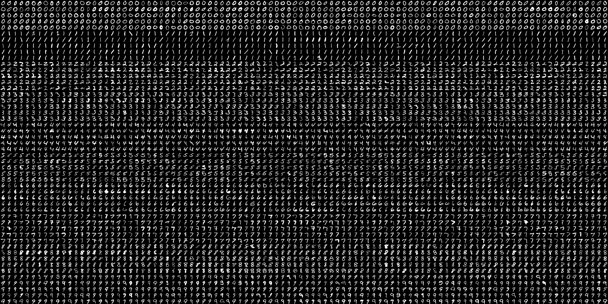
It contains 500 samples for each digit which sums up to 5000 samples in total. All we need is to extract the 20×20 images of each sample:

std::vector<cv::Mat> extractDigits(const cv::Mat &img)
{
    constexpr int digitSize = 20;
    std::vector digits;
    digits.reserve(5000);

    for(int i = 0; i < img.rows; i += digitSize)
    {
        for(int j = 0; j < img.cols; j += digitSize)
        {
            cv::Rect roi = cv::Rect(j,i,digitSize, digitSize);
            cv::Mat digitImg = img(roi);
            digits.push_back(digitImg);
        }
    }

    return digits;
}

Now, if we extract features from these digits and train a model, we can hopefully classify digits in any English document. But before this, let’s do a preprocessing to help the classifier.

­

Preprocessing

As you may have noticed, the handwritten digits are not necessarily straight. Some of them are slanted to left or right. Clearly, features of a right slanted “1” would be different from a straight “1”. To help the classifier, we can apply an Affine transformation to the slanted digits and make them straight. The Affine matrix can be estimated using moments of the image:

void deskewDigits(std::vector<cv::Mat> &digits)
{
    for (auto& digit : digits)
    {
        cv::Moments m = cv::moments(digit);

        if(abs(m.mu02) < 1e-2) return;

        float skew = m.mu11/m.mu02;
        cv::Mat warpMat = (cv::Mat_<float>(2,3) << 1, skew, -0.5*digit.rows*skew, 0, 1, 0);
        cv::warpAffine(digit, digit, warpMat, digit.size(), cv::WARP_INVERSE_MAP|cv::INTER_LINEAR);
    }
}

­

Extracting HOG features

Histogram of Oriented Gradients is one of the powerful and discriminating features that have been successfully used for several tasks such as pedestrian detection. With OpenCV, we can make an instance of cv::HOGDescriptor and call compute() function to calculate the features:

cv::Mat extractFeatures(const std::vector<cv::Mat> &digits)
{
    cv::HOGDescriptor hog(cv::Size(20,20), cv::Size(8,8), cv::Size(4,4), cv::Size(8,8), 9, 1, -1,  
                          cv::HOGDescriptor::HistogramNormType::L2Hys, 0.2, 0, 64, 1);

    const int featueSize = hog.getDescriptorSize();

    cv::Mat features(digits.size(), featueSize, CV_32FC1);

    for (int i=0; i<digits.size(); i++) 
    { 
        const auto &digitimg = digits[i];
        std::vector<float> descriptor;
        hog.compute(digitImg, descriptor);
        float* featuresPtr = features.ptr<float>(i);
        memcpy(featuresPtr, descriptor.data(), featueSize*sizeof(float));
    }

    return features;
}

Creating the dataset

Now that the features and labels of the digits are available, let’s create our dataset. OpenCV provides an easy and abstract cv::ml::TrainData for this. It allows us to shuffle the data and split it into training and testing sets via setTrainTestSplitRatio() function.

cv::Ptr<cv::ml::TrainData> createTrainData(const std::string &imgPath)
{
    cv::Mat img = cv::imread(imgPath, cv::IMREAD_GRAYSCALE);

    auto digitImages = extractDigits(img);
    deskewDigits(digitImages);
    auto features = extractFeatures(digitImages);
    auto labels = loadLabels();

    cv::Ptr<cv::ml::TrainData> data = cv::ml::TrainData::create(features, cv::ml::ROW_SAMPLE, labels);

    return data;
}

Now, 0.8 of the data (4000 digits) is devoted to training and the remaining samples (1000 digits) are devoted to testing.

­

KNN

K Nearest Neighbor is the simplest classifier in our list. Such simple that no training phase is involved! To label a new sample, it calculates its distance from all the training samples, sorts the list of the mutual distances in ascending order, and selects a label that is dominant in the first K items of the list. Note that the word “distances” refers to the Euclidean distance between feature vectors (here HOG features).

void trainKnn(const cv::Ptr<cv::ml::TrainData> &dataset)
{
    auto k_nearest = cv::ml::KNearest::create();

    k_nearest->setDefaultK(5);
    k_nearest->setIsClassifier(true);

    k_nearest->train(dataset);

    k_nearest->save("KNN.xml");
}

Normal Bayes

This classifier assumes that the distribution of the features in each class is Gaussian. In the training phase, it finds the mean and covariance of each class’s distribution, and in the testing phase, it devotes a sample to a class that has the nearest distance to its distribution.

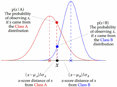
image credit to opengenus

void trainNormalBayes(const cv::Ptr<cv::ml::TrainData> &dataset)
{
    auto normal_bayes = cv::ml::NormalBayesClassifier::create();

    cv::Mat trainData = dataset->getTrainSamples();
    cv::Mat trainLabels = dataset->getTrainResponses();

    normal_bayes->train(trainData, cv::ml::ROW_SAMPLE, trainLabels);

    normal_bayes->save("NormalBayes.xml");
}

I found something strange with OpenCV’s implementation of this algorithm. Feeding the dataset object directly to the train()function results in a much less accurate model compared to a model that is trained with separate features and labels!!!

­

Logistic Regression

Despite linear regression that tries to fit a line to the data using a least-square method, logistic regression tries to fit a logistic or sigmoid function using maximum-likelihood technique. The simplicity of doing inference with this method has made it very popular among machine learning dudes. OpenCV provides functions to set the optimizer (Gradient descent and mini-batch gradient descent) as well as the learning rate and the number of iterations. To avoid overfitting, we enable regularization based on L2 norm. Note that despite other classifiers, logistic regression requires labels to be float (CV_32F) instead of int (CV_32S).

void trainLogisticRegression(const cv::Ptr<cv::ml::TrainData> &dataset)
{
    auto logistic_regression = cv::ml::LogisticRegression::create();

    logistic_regression->setLearningRate(0.001);
    logistic_regression->setIterations(100);
    logistic_regression->setRegularization(cv::ml::LogisticRegression::REG_L2);
    logistic_regression->setTrainMethod(cv::ml::LogisticRegression::MINI_BATCH);
    logistic_regression->setMiniBatchSize(100);

    cv::Mat trainData = dataset->getTrainSamples();
    cv::Mat trainLabels = dataset->getTrainResponses();
    trainLabels.convertTo(trainLabels, CV_32F);

    logistic_regression->train(trainData, 0, trainLabels);

    logistic_regression->save("LogisticRegression.xml");
}

­

Decision Trees

Decision trees can be regarded as a sequence of binary decisions that try to get close to the answer by rejecting false answers. It starts from a root node, and finishes in the leaf nodes. The nodes are extracted from the features in the training phase. The depth of the tree determines the complexity of the classifier.

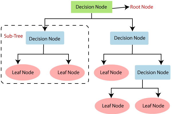
image credit to javatpoint

void trainDecisionTree(const cv::Ptr<cv::ml::TrainData> &dataset)
{
    auto decision_tree = cv::ml::DTrees::create();

    decision_tree->setMaxCategories(2);
    decision_tree->setMaxDepth(20);
    decision_tree->setMinSampleCount(1);
    decision_tree->setTruncatePrunedTree(true);
    decision_tree->setUse1SERule(true);
    decision_tree->setUseSurrogates(false);
    decision_tree->setCVFolds(1);

    decision_tree->train(dataset);

    decision_tree->save("DecisionTree.xml");
}

­

Random Forest

If we make multiple decision trees and do a majority vote on the outputs, we have a random forest algorithm. So the term “forest” comes from a collection of trees. The word “random” comes from the way that trees are trained. The training data is randomly split to N size and fed to each tree.

void trainRandomForests(const cv::Ptr<cv::ml::TrainData> &dataset)
{
    auto random_forest = cv::ml::RTrees::create();

    auto criteria = cv::TermCriteria();
    criteria.type = cv::TermCriteria::EPS + cv::TermCriteria::MAX_ITER;
    criteria.epsilon = 1e-8;
    criteria.maxCount = 5000;

    random_forest->setMaxCategories(2);
    random_forest->setMaxDepth(20);
    random_forest->setMinSampleCount(1);
    random_forest->setTruncatePrunedTree(true);
    random_forest->setUse1SERule(true);
    random_forest->setUseSurrogates(false);
    random_forest->setTermCriteria(criteria);
    random_forest->setCVFolds(1);

    random_forest->train(dataset);
    
    random_forest->save("RandomForest.xml");
}

­

SVM

Support Vector Machines are very powerful classifiers. The basic idea is to draw a line to separate the features of two classes. When features have 2, 3, or more dimensions, SVM draws a hyperplane to separate the two classes. So, SVM is originally a binary classifier (but can be easily extended to multi-class use cases). The real power of SVM comes from its kernel trick. When features are not linearly separable, the kernels (e.g. RBF) map them to a new dimension where a hyper-plane can easily discriminate them.

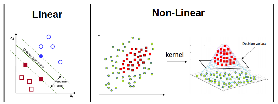
image credits to OpenCV & Grace Zhang

­

OpenCV allows us to use linear, RBF, and Sigmoid SVMs. It also allows us to find the best parameters using trainAuto() function.

void trainSVM(const cv::Ptr<cv::ml::TrainData> &dataset)
{
    auto svm = cv::ml::SVM::create();

    svm->setKernel(cv::ml::SVM::LINEAR); //cv::ml::SVM::RBF, cv::ml::SVM::SIGMOID, cv::ml::SVM::POLY
    svm->setType(cv::ml::SVM::C_SVC);

    svm->trainAuto(dataset);

    svm->save("SVM.xml");
}

­

MLP

Multi-Layer Perceptron is a widely used form of neural networks that mimic the functionality of our brain’s neurons. Each neuron gets a number of inputs, multiplies them by weights, adds a bias term, and uses an activation function to produce an output. During the training phase, the algorithm finds the optimal weights that map the inputs to the outputs.

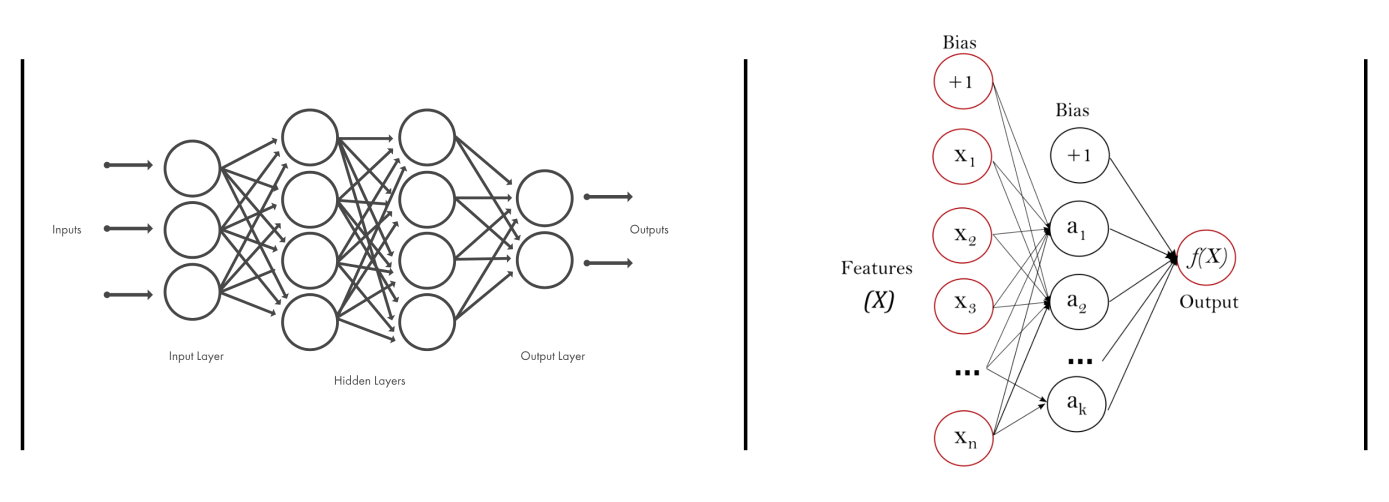
image credits to MATLAB and Scikit-learn

OpenCV provides Identity, Sigmoid, Gaussian, ReLu, and LeakyRelu activation functions. We use the classic backpropagation algorithm for training the network but you can choose RPROP or simulated annealing methods. Note that despite other classifiers that accept labels as a single column matrix, MLP requires labels to be “one-hot-encoded”. In other words, instead of [0;2;1], we should feed it with [1 0 0; 0 0 1; 0 1 0].

void trainMLP(const cv::Ptr<cv::ml::TrainData> &dataset)
{
    auto mlp = cv::ml::ANN_MLP::create();

    int nFeatures = dataset->getNVars();
    int nClasses = 10;

    cv::Mat_<int> layers(4,1);
    layers(0) = nFeatures;     // input
    layers(1) = nClasses * 32; // hidden
    layers(2) = nClasses * 16; // hidden
    layers(3) = nClasses;      // output,

    mlp->setLayerSizes(layers);
    mlp->setActivationFunction(ml::ANN_MLP::SIGMOID_SYM, 0, 0); //ml::ANN_MLP::RELU
    mlp->setTermCriteria(TermCriteria(TermCriteria::MAX_ITER + TermCriteria::EPS, 500, 0.0001));
    mlp->setTrainMethod(ml::ANN_MLP::BACKPROP, 0.0001);

    cv::Mat trainData = dataset->getTrainSamples();
    cv::Mat trainLabels = dataset->getTrainResponses();
    trainLabels = oneHotEncode(trainLabels, nClasses);

    mlp->train(trainData, cv::ml::ROW_SAMPLE, trainLabels);

    mlp->save("MLP.xml");
}

cv::Mat oneHotEncode(const cv::Mat& labels, const int numClasses)
{
    cv::Mat output = cv::Mat::zeros(labels.rows, numClasses, CV_32F);

    const int* labelsPtr = labels.ptr<int>(0);

    for (int i=0; i<labels.rows; i++)
    { 
        float* outputPtr = output.ptr<float>(i);
        int id = labelsPtr[i];
        outputPtr[id] = 1.f;
    }

    return output;
}

­

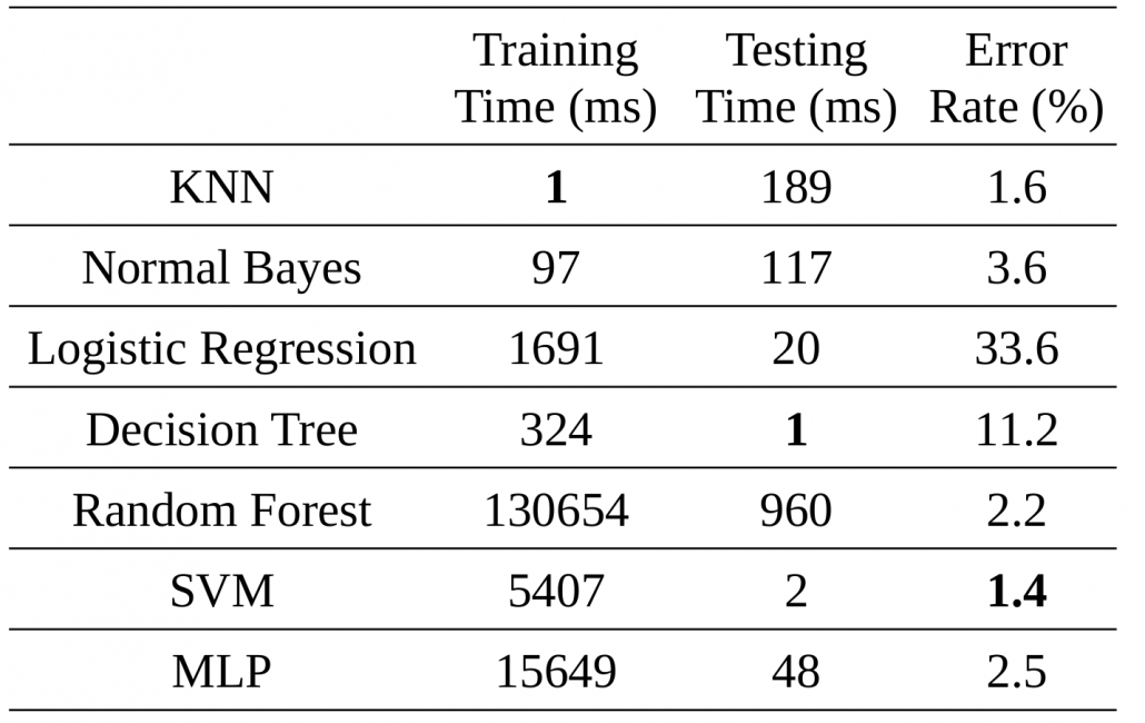
Putting it all together

The following table compares training and testing time, as well as error rate of the mentioned models. Note that:

1. We just studied the task of handwritten classification with HOG features. It is highly probable that the behavior of these classifiers on other datasets with different features would be different.
2. I didn’t tweak the parameters of each model. Maybe by some tweaking, we get different accuracies.

Let’s do it with a CNN

All the mentioned algorithms required features to work. If we feed them with better and more discriminating features, we will get higher classification accuracies. But designing good features (also known as feature engineering) is not easy. In the next post, we will see how a simple Convolutional Neural Network can achieve superb accuracies without the need to give handcrafted features. Stay tuned.