Cascade classifier is an old algorithm which was originally proposed for real-time face detection on CPUs. In this post, I will cover it’s nice and powerful idea, and then in the next post give you some clear instructions to easily train an accurate custom object detector using my C++ toolbox.

1. Why cascade classifier?

You must have heard about YOLO and SSD. They are state of the art CNN-based object detectors that can handle multiple classes of objects with different poses (like cats and dogs) in complex backgrounds. So they are very good in overall. But there might be some situations where we can detect the desired objects using simpler methods. Cascade classifier, proposed by Viola and Jones, is one of those simpler methods which can provide surprisingly good accuracies if the objects are rigid. Compared to CNNs, cascades require fewer data and are potentially faster to train and execute. So:

• if your objects are rigid (i.e. their aspect ratio doesn’t change),

• if you are looking for an efficient detector to deploy on ARM CPUs, and

• if you don’t have tons of images for training,

then I recommend you to go with cascade classifiers which are implemented in OpenCV.

2. Workflow

For now, consider cascade as a black-box classifier. Given this classifier, first, a pyramid is constructed from the input image (because we need multi-scale detection). Then a sliding window scans each sub-level image and the classifier returns the regions that contain the desired object. Since an object might be detected in multiple sliding windows/scales, non-maximum suppression is applied to remove redundant boxes.

But how exactly the classifier works? What are the features? Why it is called cascade? And how such a sliding window strategy can run efficiently? We will find the answers in a few minutes.

3. How does it work?

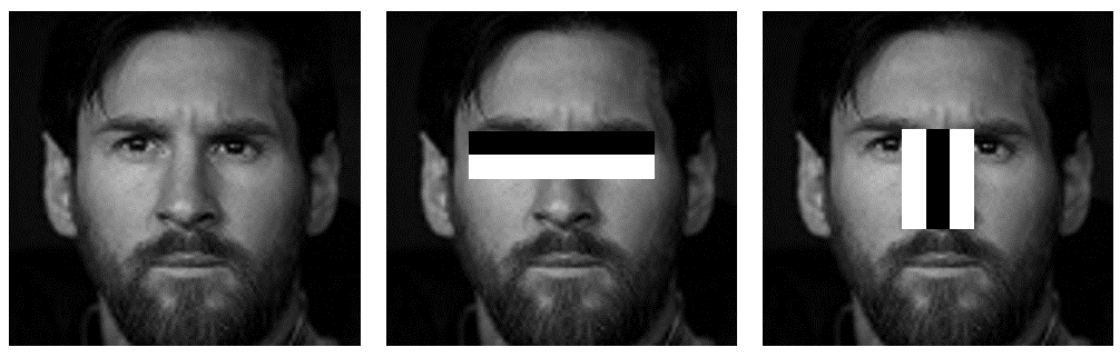
Suppose we want to detect face. Face has some general properties. For example, nose is brighter than its left and right regions. Lips make contrast with left, right, top, and bottom. Eyes are darker regions than their surrounding regions, and etc. If we can measure these properties, then we can feed them to a classifier to decide whether it is face or not.

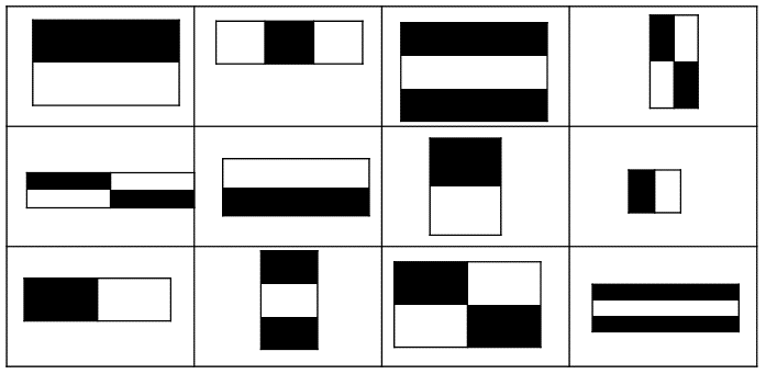
3.1 Haar-like features

Haar-like features can measure these properties for us. The value of each feature is calculated by subtracting the sum of all pixels under the black regions from the sum of all pixels under the white regions.

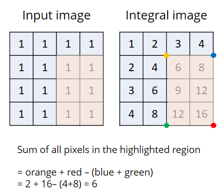
3.2 Integral image

The above figure shows a few numbers of the features used by the algorithm. In real, there are many many more features. To evaluate the value of each one of these features, sum of all the pixels under the black and white regions must be calculated. This is very slow. The authors proposed a nice idea to accelerate this part. They called it “integral image”. We make the integral image beforehand and then query the sum of all pixels in a region only by doing 2 additions and one subtraction. This way, we can query thousands of regions with a few computational overhead.

3.3 Feature reduction and Classification

One can define hundreds and thousands of Haar-like features simply by rotating, scaling, and a bunch of other geometric transformations.

Evaluating all these features (even with integral image) takes time. The authors have used Adaboost to remove redundant features. Adaboost is a learning algorithm that produces a strong classifier from a linear combination of multiple weak classifiers.

The weak classifiers are often single layer decision trees (also called stumps). They are very fast to execute. So, Adaboost is a combination of weak-but-fast classifiers which form an accurate-but-still-fast classifier when working together. A feature is considered okay to be included if it can at least perform better than random guessing (detects more than half the cases).

3.4 Cascading

Cascading lets the algorithm to quickly reject non-face regions and spend more time on regions with potential faces. Look at the figure. There are a number of stages each with an Adaboost classifier. The complexity of the Adaboost classifier grows with the number of the stage. The first stages have simple classifiers which can quickly reject non-face regions. The last stages have complicated classifiers to ensure high true positive rates.

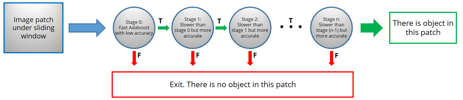
It is very important that each stage has a very low false negative rate. Because if a face would be wrongly classified as non-face, it is removed forever and there is no chance to correct it later. However, each stage can have a high false positive rate because the mistakes can be corrected in subsequent stages.

4. A simple example in OpenCV

OpenCV has implemented cascade classifiers. They have trained some models for detecting face, eye, and body which are downloaded in the “data” folder when you download the OpenCV. The following code shows a simple way to use the face model.

#include <opencv2/opencv.hpp>

using namespace std;
using namespace cv;

int main()
{
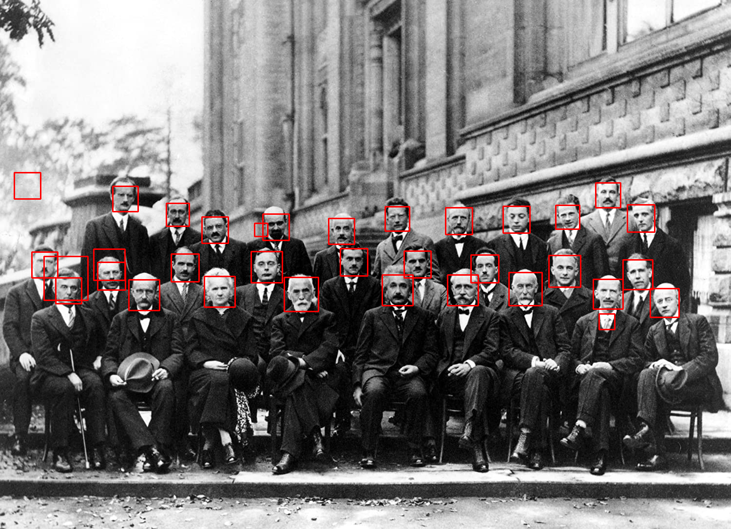
    Mat img = imread("solvay_conference_1927.jpg");

    CascadeClassifier detector("haarcascade_frontalface_default.xml");

    vector<Rect> faces;
    detector.detectMultiScale(img, faces);

    for (const auto& face:faces)
        rectangle(img, face, Scalar(0,0,255), 2);

    imshow("Faces", img);
    waitKey(0);

    return 0;
}

A CascadeClassifier object is constructed and the .xml model is loaded. Then detectMultiScale applies the model over the image and returns the objects. You can read OpenCV’s document for further information.

5. Want to train your custom model?

Read the next post.